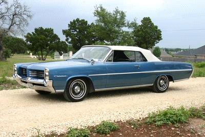
I recently had a request to do some image analysis and to isolate certain elements of the image. In this case, the request was to isolate cars. Any given pixel in the image that is “not car” should be converted to a black pixel and any pixel that is part of a car should be white. As an example, for this image:
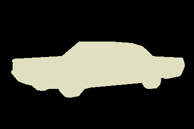
The desired output is:
Initially, we were thinking that this might be a good problem for “crowdsourcing” and we could set up some MTurk’s HIT’s to have people select the image. However, after some thought, I decided to see what Mathematica could do for us with this problem. As it turns out, it can do a lot!
Let’s start by establishing some definitions.
“Image Segmentation” is a partition of an image into several “coherent” parts, but without any attempt at understanding what any of these parts represent. One of the most referenced papers (but not the first) is Shi and Malik “Normalized Cuts and Image Segmentation” PAMI 2000. This paper tries to define “coherence” in terms of low-level cues such as color, texture, and smoothness of boundary.
“Semantic segmentation” attempts to partition the image into semantically meaningful parts, and to classify each part into one of the pre-determined classes. You can also achieve the same goal by classifying each pixel rather than the entire image. In that case, you are doing pixel-wise classification, which leads to the same result but taking a different path.
So, “semantic segmentation”, “scene labeling” and “pixel-wise classification” are basically trying to achieve the same goal-semantically understanding the role of each pixel in the image. We can take many paths to reach that goal, and these paths have slight nuances in the terminology.
Out of the box, the latest version of Mathematica comes with broad Neural Network Repository including a set of Semantic Segmentation pre-trained models, which we will be using to solve our problem.
Using one of the Neural Networks is quite easy. The first time you evaluate a NetModel, it downloads a fairly large amount of data from the internet so it will take a while to run the first time. We’ll use the Ademxapp Model A1 Trained on ADE20K Data.
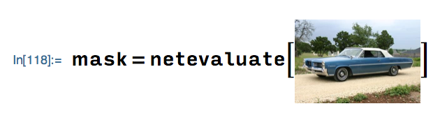
First, we’ll have to set up a function to deal with resizing and reshaping the input. Basically, the network has been trained on images of certain sizes and types, so this function changes the input image into the size and type the neural network is expecting.
netevaluate[img_, device_: "CPU"] :=
Block[{net, resized, encData, dec, mean, var, prob},
net = NetModel["Ademxapp Model A1 Trained on ADE20K Data"];
resized = ImageResize[img, {504}];
encData = Normal@NetExtract[net, "Input"];
dec = NetExtract[net, "Output"];
{mean, var} = Lookup[encData, {"MeanImage", "VarianceImage"}];
prob = NetReplacePart[
net, {"Input" ->
NetEncoder[{"Image", ImageDimensions@resized,
"MeanImage" -> mean, "VarianceImage" -> var}],
"Output" -> Automatic}][resized, TargetDevice -> device];
prob = ArrayResample[prob, Append[Reverse@ImageDimensions@img, 150]];
dec[prob]]
Then, we create a list of labels, one for each class that the neural network knows about. This is in the documentation for each Neural Network. You would expect that it would be easy enough to include these labels in the model instead of having to declare them. I suspect that the reason you are asked to specify the labels is so that you can shorten the list if you know ahead of time that certain objects will not be present in the image and that will improve the accuracy of the results.
labels = {"wall", "building", "sky", "floor", "tree", "ceiling", "road", "bed", "windowpane", "grass", "cabinet", "sidewalk", "person", "earth", "door", "table", "mountain", "plant", "curtain", "chair", "car", "water", "painting", "sofa", "shelf", "house", "sea", "mirror", "rug", "field", "armchair", "seat", "fence", "desk", "rock", "wardrobe", "lamp", "bathtub", "railing", "cushion", "base", "box", "column", "signboard", "chest", "counter", "sand", "sink", "skyscraper", "fireplace", "refrigerator", "grandstand", "path", "stairs", "runway", "case", "pool", "pillow", "screen", "stairway", "river", "bridge", "bookcase", "blind", "coffee", "toilet", "flower", "book", "hill", "bench", "countertop", "stove", "palm", "kitchen", "computer", "swivel", "boat", "bar", "arcade", "hovel", "bus", "towel", "light", "truck", "tower", "chandelier", "awning", "streetlight", "booth", "television", "airplane", "dirt", "apparel", "pole", "land", "bannister", "escalator", "ottoman", "bottle", "buffet", "poster", "stage", "van", "ship", "fountain", "conveyer", "canopy", "washer", "plaything", "swimming", "stool", "barrel", "basket", "waterfall", "tent", "bag", "minibike", "cradle", "oven", "ball", "food", "step", "tank", "trade", "microwave", "pot", "animal", "bicycle", "lake", "dishwasher", "screen", "blanket", "sculpture", "hood", "sconce", "vase", "traffic", "tray", "ashcan", "fan", "pier", "crt", "plate", "monitor", "bulletin", "shower", "radiator", "glass", "clock", "flag"};
Notice that the 21st element in the list is “car”. This means that this network is capable of recognizing cars. We can now create a mask that segments all the objects in the image that the neural network can recognize.
You can visualize this mask easily by using Colorize
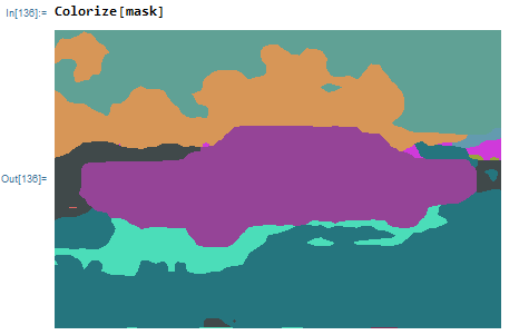
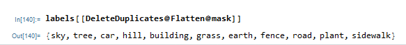
Also, you can easily get a list of all the items the neural network identified: with labels[[DeleteDuplicates@Flatten@mask]]
Now that we have this mask, we can get rid of all the types of objects that aren’t the kind we’re trying to identify—in our case, cars.
First, we find the index of the object we’re looking for in the labels.
index = Position[labels, "car"]
In the case of this network, it’s 21. Now we set all the pixels in the mask to be 0 unless they have the magic value of 21.
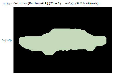
I didn’t try out all the segmentation models that come with Mathematica to appreciate the difference in the results for different models. Feel free to try them out yourself and share your results with me. Enjoy.